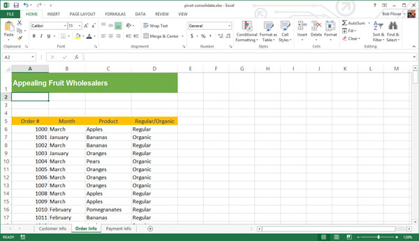
Advanced PivotTables: Combining Data from Multiple Sheets ~ Kimliang Mich (All4Free)

When you want to create a PivotTable, what do you do if you have data in different worksheets? If you’re using Excel 2013, you have a streamlined method of doing this. There’s a technique called the Data Model, and it uses data relationships the way a database does.
In this tutorial, I'll show you everything you need to make a PivotTable in Excel 2013 from data in multiple sheets, using the Data Model.

Screencast

If you want to follow along with this tutorial using your own Excel file, you can do so. Or if you prefer, download the zip file included for this tutorial, which contains a sample workbook called Pivot Consolidate.xlsx.

Examining the Data

This workbook has three worksheets: Customer Info, Order Info, and Payment Info.
Click the Customer Info sheet, and see that it contains order numbers and the name and state of customers.

Click the Order Info sheet, and see that it also contains order numbers, as well as fields for the month, the products ordered, and whether or not the products are organic.

Click the Payment Info sheet, and see that it contains order numbers, the dollar amount of each sale, the payment method, and whether the order was placed by a new or an existing customer.

By connecting all these sheets inside the PivotTable’s task pane, we can selected data from each of the sheets. Since the order numbers exist in all three sheets, they will become the connection points. This is what a database calls a primary key. Note that it isn’t always necessary to have a primary key, but it reduces the chance of error.

Create Named Tables

Before creating the PivotTable, let’s create a table from each of the sheets.
Click back on the Customer Table, then click anywhere inside the data area. Go to the Insert tab of the ribbon bar, then click the Table icon.

creating a table from existing data — Convert data on a worksheet by selecting **Insert > Table**

The Create Table dialog box correctly identifies the area of the table. The checkbox on bottom should also identify that the first row of the table is for headers. (If not, select that option.)

Click OK, and now you have a table with striped shading and filter buttons. You can click inside it to deselect, if you want a better look at it (just don’t click outside the table). The ribbon bar also displays a Design tab for the table. On the left side of the ribbon, the Table Name box shows a temporary name of Table1. Delete that, and call it Customer_Info (use an underscore instead of a space). Then press Enter.

applying a name to a table — Apply a name to each table

Repeat this process on the Order Info and Payment Info sheets. Call the tables Order_Info and Payment_Info, respectively.
Now we’re ready to insert the PivotTable.

Inserting the PivotTable

On the Payment Info sheet, make sure the cursor is somewhere in the table. Go back to the Insert tab of the ribbon, and click the PivotTable icon (it’s the very first icon).

The dialog box that appears should correctly identify the table and select that the PivotTable will go on a new worksheet. On bottom, click the check box for Add this data to the Data Model. Then click OK.

add data to the Data Model — Adding the data to the Data Model is what allow the connections to work

You’ll now have a PivotTable on a new worksheet, there will be a task pane on the right side of the screen, and the ribbon bar will display the Analyze tab.
The task pane shows the table and fields of just the active sheet, so click ALL to see all the tables that you created. But before we can use them, we have to connect them to each other, and that means creating relationships. Click the Relationships button on the ribbon bar.

Setting Up Table Relationships

Clicking that button displays the Manage Relationships dialog. Click the New button, and that displays the Create Relationship dialog. We’ll create two relationships using the Order # field as the connector.
From the drop-down lists, choose Payment_Info for the table, and next to it, pick Order # from the Column drop-down. On the second row, choose Customer_Info from the Related Table drop-down list, and next to it, pick Order # from the Related Column drop-down list.

creating a table relationship — There are three tables, so create two relationships

This means the Payment_Info and Customer_Info tables are related where they have matching order numbers.
Click OK, and we see that relationship listed in the Manage Relationships box.
Repeat this process to create a relationship that joins Payment_Info to Order_Info, also using the Order # field. The Manage Relationships box should now look like this:

list of all relationships — The Manage Relationships dialog will display the relationships that you create

Note that it isn’t necessary to create a relationship between the Order_Info and Customer_Info tables, since they’re joined automatically through the Payment_Info table.
Click the Close button at the bottom of the box. Now we can finally drag fields into the PivotTable.

Inserting Fields Into the PivotTable

In the ALL section of the task pane, click the small arrows to twirl open the three tables, so you see their fields. Drag fields into the PivotTable areas as follows:

State and Month into rows
Product into columns
$ Sale into values
Status into filters

final PivotTable — Drag fields from each of the three tables into the PivotTable

You can now use and modify this like any other PivotTable.

Conclusion

Using the new Object Data Model feature in Excel 2013, you can cherry-pick fields from multiple worksheets to create a unified PivotTable. Keep in mind that the rows of each table need to be related to each other in some way. You’ll have the best chance of success when the tables have a common field with unique values.